The Paradox of Naive Bayes: When Simple Becomes Sophisticated

DATA SCIENCE THEORY | NAIVE BAYES | MACHINE LEARNING

The Paradox of Naive Bayes: When Simple Becomes Sophisticated

A theoretical intro that shows how its theoretical elegance, practical efficiency and effectiveness continue to make it a valuable tool for ML practitioners

To read this article for free click here.

Naive Bayes presents an interesting puzzle in machine learning; an algorithm that performs far better than its simple premise would suggest. While advanced algorithms like Support Vector Machines and Decision Trees create complex category boundaries, Naive Bayes uses a simpler approach: it calculates the most likely outcome based on the available evidence.

This simplicity has proven remarkably effective. Take Gmail’s spam filter, one of the most widely used machine learning applications. In its early implementation, Google chose Naive Bayes over more sophisticated alternatives. The choice paid off; the algorithm effectively identified spam emails and could quickly adapt to new spam tactics, processing millions of messages each day.

Naive Bayes probabilistic foundation makes it particularly useful in situations involving uncertainty. From email filtering to medical diagnosis and customer feedback analysis, Naive Bayes continues to deliver reliable results. It stands as proof that in machine learning, complexity isn’t always the answer.

Understanding Naive Bayes Through Restaurant Reviews

Imagine you’re a food critic trying to predict whether a restaurant will be good based on reviews. You notice certain words appear more frequently in positive reviews (‘delicious’, ‘fantastic’, ‘wonderful’) versus negative ones (‘disappointing’, ‘mediocre’, ‘bland’). This is exactly the kind of pattern that Naive Bayes excels at identifying.

How does it actually work? Think of Naive Bayes as calculating the likelihood of a review being positive or negative in two steps. First, it learns from training data: for each word, it calculates how often that word appears in good and bad reviews. For example, ‘delicious’ might appear in 80% of good reviews but only 5% of bad ones. Second, when it sees a new review, it combines these learned probabilities to make its prediction.

The ‘naive’ part of Naive Bayes comes from a seemingly problematic assumption: it treats each word as independent of the others. Consider the phrase ‘not delicious’ in a restaurant review. In reality, these two words combine to create a clearly negative sentiment. However, Naive Bayes would by definition process them as separate independent tokens ‘not’ and ‘delicious’. The algorithm might see ‘delicious’ as a positive indicator and ‘not’ as a relatively neutral word potentially missing their combined negative meaning. This is the essence of the ‘naive’ assumption, it deliberately ignores how words work together to create meaning. Despite this, it works surprisingly well.

The ‘Bayes’ in Naive Bayes comes from Bayes Theorem, a key concept in probability theory. Using our restaurant example, instead of directly asking ‘Is this a good restaurant based on these words?’, it flips the question to ‘How likely are we to see these words in good restaurant reviews?’ By combining these probabilities with how common good restaurants are in general, it can predict whether a new review is probably positive or negative.

The brilliance of Naive Bayes lies in its simplicity. Despite, or perhaps because of, its basic assumptions this straightforward algorithm keeps delivering remarkable results. It is a useful reminder that while modern machine learning veers towards complexity, often the simplest approach is exactly what we need.

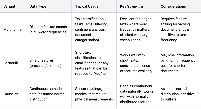
The Three Common Variants of Naive Bayes

Naive Bayes comes in three commonly used variants each suited to different types of data and classification tasks. Multinomial Naive Bayes and Bernoulli Naive Bayes both work with discrete features, typically text, and utilise a lexicon approach, where the lexicon is built through supervised model training. Multinomial handles frequency counts of features (like word occurrences in text or pattern frequencies in images), while Bernoulli focuses on simply binary presence/absence of features. Gaussian Naive Bayes differs by working with continuous numerical data, assuming features follow a normal distribution, making it suitable for measurements like sensor readings or physical attributes.

Data Pre-processing & Model Training: The Lexicon

The effectiveness of Multinomial and Bernoulli Naive Bayes hinges on how well they understand and process words and linguistic patterns.

As supervised learning algorithms, Naive Bayes needs labelled examples to learn from. Each example helps build a comprehensive lexicon through several crucial preprocessing steps:

The text is first converted to lowercase and stripped of punctuation. Common stop words like “the” and “and” are removed, as they occur frequently but add little value.

Text analysis gets messy when dealing with different forms of the same word. A simple task like scanning customer feedback could treat ‘analyse’, ‘analysed’, ‘analysing’, and ‘analysis’ as completely different words when they are all expressing the same thing.

There are two main tools to handle this, stemming or lemmatisation. Stemming is the quick and dirty approach, chopping words down to their root form, turning ‘analysing’ into ‘analys’. It’s crude but fast often creating word stems that look a bit odd. Lemmatisation takes a more careful approach, converting words to their proper dictionary form, turning ‘analysing’ into ‘analyse’. It’s more accurate but takes more computing power. Both individual words and word sequences (N-grams) are included to capture meaningful phrases.

The choice between them depends on your needs. If you are building a quick prototype or speed is crucial, stemming might be good enough. For applications where accuracy really matters, like legal document analysis, lemmatisations precision could be worth the extra processing time.

TF-IDF (Term Frequency-Inverse Document Frequency) adds another vital layer. This technique helps identify the most meaningful words for classification, and reduces the weights of common terms. In technical support, for example, while ‘error’ might appear frequently across all queries, more specific terms like ‘password’ or ‘database’ often prove more useful for classification.

Very rare terms (often typos) and extremely common words are typically removed creating a focused vocabulary of the most relevant features. This shouldn’t be seen as just fine-tuning as it is often what separates an average classifier from an excellent one.

The lexicon should also evolve with time. New product names, technical terms, and changing customer language patterns mean regular retraining or updates. Many organisations schedule regular lexicon reviews to keep their Naive Bayes classifiers current. Naive Bayes can update incrementally (e.g., adjust weights as new labelled data arrives) without full retraining. This gives Naive Bayes a key advantage over other algorithms such as Neural Networks.

Working with Related Features in Naive Bayes

The core assumption of Naive Bayes, that all features are independent, is clearly wrong in the real world. Words in language obviously relate to each other, as do medical symptoms and sensor readings. The real skill lies in knowing when this simplification matters.

Mostly this oversimplification doesn’t cause problems. In text analysis, treating ‘New’ and ‘York’ as independent words rarely affects your results significantly. However, in medical diagnosis treating a patients blood pressure and heart rate as completely unrelated could lead to dangerous conclusions.

To handle this, practitioners carefully prepare their data before training the model. They might combine related measurements, for example merging blood pressure and heart rate into a single ‘cardiovascular health’ score. This way, they build their medical knowledge into the data structure itself.

This approach helps explain why Naive Bayes still works well in medical applications like symptom screening. While the algorithm itself doesn’t understand how features relate to each other, careful preparation of the input data, like grouping connected symptoms or measurements, helps overcome this limitation. The key is thoughtful data preparation rather than relying on the algorithm to work out these relationships itself.

Multinomial Naive Bayes

Multinomial Naive Bayes works like a word counter that remembers class context. For each class (like spam/not-spam), it keeps track of how often each word from the lexicon appeared in training documents of that class. When classifying a new document it looks at each words frequency in the document and multiplies the probabilities based on how often those words appeared in each class during training. For example, if ‘money’ appeared frequently in spam emails during training, finding multiple instances of ‘money’ in a new email would strongly increase its spam probability.

Bernoulli Naive Bayes

Bernoulli Naive Bayes instead works like a checklist. For each class it remembers what percentage of training documents contained each word from the lexicon (this time ignoring how many times the word appeared). When classifying a new document it checks off which words are present and multiplies probabilities based on how often those words appeared in documents of each class during training. Importantly, it also factors in the absence of words; if certain words typically appear in legitimate emails but are missing, that affects the probability too. So if words like ‘meeting’ or ‘report’ are common in legitimate emails but absent from a new email, that could increase its spam probability.

Gaussian Naive Bayes

While Multinomial and Bernoulli variants work with words and counts, Gaussian Naive Bayes handles continuous numerical data through a similar pattern-matching approach. During training, it learns the typical range and spread of values for each feature within each class. Think of it as building a statistical profile rather than a word-based lexicon.

For each feature Gaussian Naive Bayes calculates two key values per class: the mean (average) and variance (spread) of the measurements. It assumes these values follow a normal distribution where most measurements cluster around the middle. For example, in quality control:

• A properly functioning machine might typically produce parts 10mm long with a variance of 0.1mm
• A faulty machine might produce parts averaging 10.5mm with a variance of 0.3mm

When classifying new data, the algorithm calculates how likely each measurement would be under these different distributions. It combines these probabilities across all features, just as lexicon-based methods combine evidence from different words.

Gaussian Naive Bayes also makes the ‘naive’ assumption that features are independent. In reality, measurements like height and weight are obviously related, but once again the algorithm treats them as separate pieces of evidence. And it works.

The Zero Probability Problem

When Naive Bayes encounters new words during testing that were not in its training data, it would normally assign them a zero probability. This can be disastrous; as this means a single previously unseen word could make the model completely ignore all other evidence. Laplace smoothing (also called add-one smoothing) solves this by adding a small count to every feature, including those we haven’t seen. Think of it as saying “well, just because we haven’t seen it before doesn’t mean it’s impossible.” This gives unseen features a small but non-zero probability, preventing them from ruining the entire classification.

The Future of Naive Bayes in Machine Learning

While deep learning and transformer models have revolutionised many areas of machine learning, Naive Bayes maintains its relevance through key advantages. Its probability-based approach offers clear interpretability. Data Scientists can examine exactly why a classification was made by looking at the contributing probabilities from each feature. This transparency, combined with its computational efficiency, makes it really valuable in applications requiring explainable decisions or real-time processing. This interpretability is particularly crucial in sensitive domains like healthcare or financial services, where understanding the reasoning behind classifications is often as important as the classifications themselves.

Moreover, Naive Bayes adapts well to hybrid approaches, whether as part of an ensemble, as a feature generator for deep learning models, or in combination with other algorithms. Its probabilistic outputs can serve as valuable features for more complex models, while its speed and efficiency make it an excellent candidate for initial data exploration and baseline model development. As machine learning continues to evolve, the need for efficient, interpretable models that can work with limited data and computational resources ensures that Naive Bayes and its variants will remain valuable tools in the machine learning toolkit.

Looking ahead, Naive Bayes is likely to find new applications in emerging fields like edge computing and IoT devices, where its computational efficiency and minimal resource requirements make it an attractive choice. Its ability to handle incremental updates and adapt to changing data patterns also positions it well for streaming data applications and online learning scenarios.

The success of Naive Bayes reminds us that sometimes the most elegant solutions are also the simplest. Its combination of theoretical elegance, practical efficiency, and surprising effectiveness continues to make it a valuable tool for modern machine learning practitioners, proving that being ‘naive’ can sometimes be surprisingly sophisticated.

Visit my Naive Bayes Demo App Here.

Jamie is founder at Bloch.ai, Visiting Fellow in Enterprise AI at Manchester Metropolitan University and teaches AI programming with Python on the MSc AI Apprenticeship programme with QA & Northumbria University. He prefers cheese toasties.

Follow Jamie here and on LinkedIn: Jamie Crossman-Smith | LinkedIn